MktModel
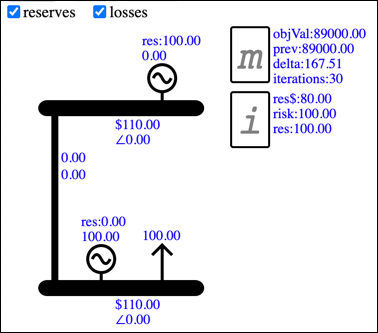
MktModel is a browser-based app for building and solving an Electricity Market Model. An example model that has been built and solved looks like this:
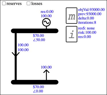
Build and Solve
The following frame contains the MktModel app. You can build and solve the simple model shown above by clicking the buttons Bus-Bus-Br-Gen-Ld to add Components to the Model and then click Solve, which will solve the Model using the default properties of the Components:
The full-screen experience is available
here
The following sections provide an introduction to electricity market modelling, using the MktModel app to build and solve examples.
Mathematical Model
The results shown above are produced by solving a mathematical model that is based on the displayed Components. The mathematical model is a set of constraints, built by automatically combining the Components with corresponding mathematical model definitions. You can see the mathematical model definitions on the Main - Model Def display.
In the electricity market model, the constraints model the characteristics of the network and the market. For example the nodeBal constraint enforces that the flow of electricity into a Bus is equal to the flow out. The enOffertTrancheLimit constraint models the upper limit of a Generator's offer tranche. Once the model is solved you can view a Component's constraints on its Data page.
Objective Value
In addition to the constraints that define the system being modelled, there is a constraint which implements the objective function to calculate the objective value. When the model is solved, the solver maxmises the objective value while obeying the limits of the other constraints.
Because the app has every constraint associated with a displayed Component, the objective function is associated with a Mathematical Model Component, m, which is automatically added to every model. The other Component that is added automatically is the Island Component, i, which represents the electrical island, this is used when modelling reserves as described later.
Solving the Model
The mathematical model definitions and the Component details are sent to the solver. You can see what is sent by looking at the display Main - JSON Model.
The solver is bespoke code written in SCALA, running on the Heroku platform.
The first part of the SCALA code is the controller which receives the JSON from the webpage, extracts the model elements and the constraint definitions, and uses these to build the mathematical model:
SCALA Controller
After building the model, the following procedure is called to solve the model using the simplex algorithm:
SCALA Simplex Solver
After the result is returned you can see the constraints that the solver built by selecting a Component and then clicking the Data button.
Objective Function
When the model is solved, the simplex algorithm determines quantities for the variables in the constraints, such that the objective value is maximised. The objective value is calculated by the objective function, which can be viewed on the Data page of the Mathematical Model Component:
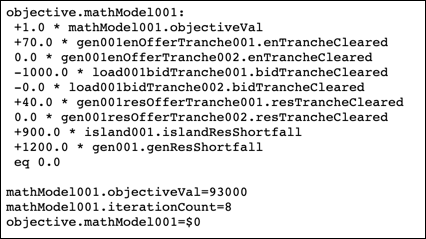
The objective value is calculated as the value of the load bids that are cleared, less the cost of the offers that are cleared. Based on this the solver would like to clear all of the bids and none of the offers, but is prevented from doing so by the constraints of the model. For example the node balance constraint requires that the flow into a Bus is equal to the flow out. The bids represent flow out of the Bus so for them to clear, electricity must flow into the Bus. This inward flow must be from either offers cleared at the Bus, or Branch flow from some other Bus where offers have cleared. Other constraints such as the tranche limits of the bids and offers, or the flow limit on the branch, must also be observed.
Binding constraints and shadow prices
If a constraint in some way prevents the objective value from increasing, then that constraint is said to be binding and has an associated non-zero shadow price. The shadow price represents the rate of increase in the objective value that would occur if the constraint was relaxed, i.e., not strictly enforced.
Throughout the solve the simplex algorithm is keeping track of the objective-value impact of each constraint and then adjusting the variables in the model in order to assist the constraint that is most valuable. At some point none of the constraints can be improved without breaking some other constraint, the solve is finished and the quantities can be extracted from the value of the variables. The shadow prices can be extracted from the value associated with relaxing the constraints.
Explaining prices
The bus price is set by the shadow price of the node balance constraint, so we can explain the bus price by mimicing the effect of relaxing the node balance constraint. Because the node balance constraint enforces that electricity flow into the bus is equal to flow out, the constraint is relaxed by allowing more electricity to enter or leave the bus, without any associated cost. To demonstrate this, first build and solve the following model:
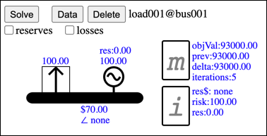
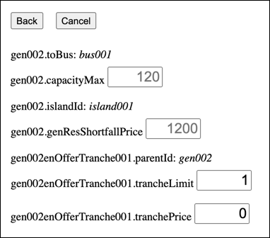
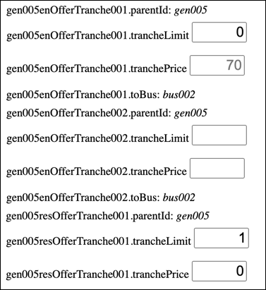
The bus price is $70. To mimic relaxing the node balance constraint, we will allow 1MW of energy to arrive at the bus for free. To do this, add a Generator to the Bus...
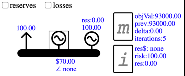
...and edit its data so that its energy tranche has a limit of 1 and a price of $0:
When this model is solved...
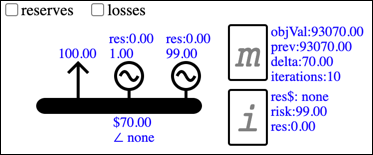
...the objective value has a delta of $70, which represents the impact of relaxing the node balance constraint. The objective value is the sum of cleared bids, less the cost of cleared offers, and we can see that the $70 increase was the result of a 1MW decrease in cleared $70 offers (you can check this via the objective function on the Model Component's Data page m).
Because this shows that the value of energy at this bus is $70, any energy offer will only clear if its cost is <= this $70 benefit.
This is a fairly straight forward example, but later we will use the same procedure to explain the reserve price, which is not so intuitive (to be added).
Adjusting the Network
The next example builds a network that requires adjusting the location of the Components. To move a Component, click to select it and then drag anywhere on the screen. For a Bus or Branch if the drag direction starts parallel to the length then it will resize the Component, a drag that starts perpendicular will move the Component.
Spring Washer Effect
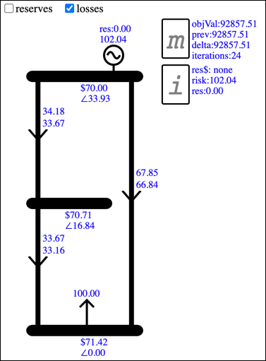
The Spring Washer Effect can cause negative prices. To demonstrate this, build and solve the following model:
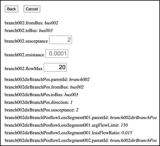
As shown on the Data page below, the powerFlow Constraint links the branchFlow Variable of the Branch to the phaseAngle Variable of the Bus. The linking factor is the Branch susceptance property, currently set at the default value of 2.0:
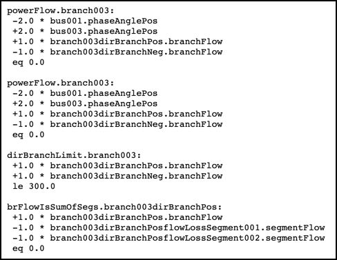
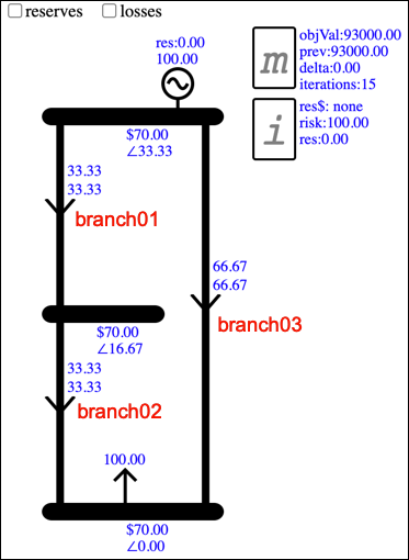
In the example shown above, the location of the Generation and Load result in phase angles that force the flow on Branch03 to be the sum of the flow on the other two Branches.
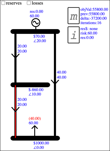
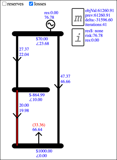
Now edit the properties of Branch02 to limit its flowMax to 20:
This causes Branch02 to bind, resulting in the spring-washer effect, with a negative energy price of -$860 at Bus02:
Explaining the Spring Washer price
The Bus price is the shadow price of the nodeBal Constraint, which constrains flow into the Bus to be equal to flow out. The price at Bus03 is $1000. This is because there are uncleared $1000 bids at this Bus. Relaxing the node balance Constraint would allow another unit of $1000 bids to clear.
The price at Bus02 is -$860. The negative price indicates that there is a benefit to less energy at this Bus, i.e., extra load, rather than extra generation. To demonstrate how extra load provides a benefit, add a Load to Bus02 and edit its Data to set the tranchLimit to 1 and tranchePrice to 0:
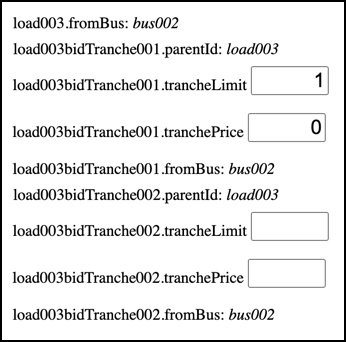
As shown below, the increased load at Bus02 allows the flow on Branch01 to increase by 1.0 while maintaining Branch02 at its limit of 20. This allows the Branch03 flow to increase by 1.0, allowing more load bids to clear at Bus03:
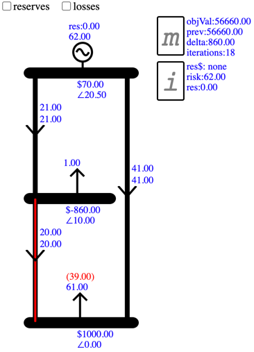
The change in the Objective Value is $860, which matches the Bus02 price, and we can confirm this by calculation:
Benefit from increasing cleared $1000 bids to 61MW:
(61 - 60) * $1000 = $1000
Cost from increasing cleared offers by 2MW to cover 1MW dummy load and 1MW cleared bids:
(72 - 70) * $70 = $140
Benefit - Cost: $1000 - $140 = 860
Overall the benefit of the extra cleared bids outweighs the cost of the extra cleared offers, thus demonstrating the benefit of load at Bus02.
Non-physical losses
With losses enabled and before the binding constraint is applied, i.e., before the limit on Branch02 is lowered to 20, the Spring Washer model looks like this:
After the binding constraint is applied and the Spring Washer Effect occurs, the result is shown below. Before the Spring Washer Effect the losses on Branch01 were less than 1 unit, but afterwards they are over 5. This is because extra losses have a similar effect to extra load at Bus02... they allow extra flow on Branch01 which allows extra flow on Branch03 and more load bids to clear.
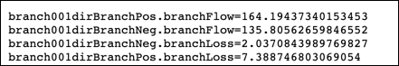
The solver is able to increase the losses on Branch01 because branch flow is modelled as forward and reverse directional branches, which is done because the solver requires all Variables to be positive. The overall Branch flow is the forward direction flow minus reverse direction flow. Because both directions have losses associated with flow, and losses have a cost due to the generation required to supply them, normally only one direction has non-zero flow. When the Spring Washer Effect occurs and the benefit of losses outweighs the cost, the solver schedules flow in both directions. As shown on the Data page for Branch01, the overall flow is the result of large forward and reverse flows:
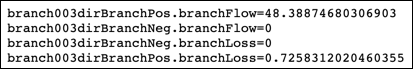
The results for Branch03 only show positive flow, because for Branch03 losses have no benefit, only cost:
The extra losses on Branch02, i.e., those over and above an accurate modelling of the losses that would physically occur on a Branch with that flow, are referred to as non-physical losses.
Reserves
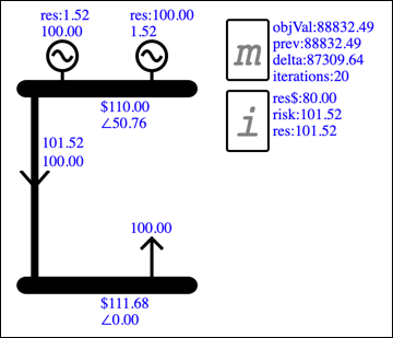
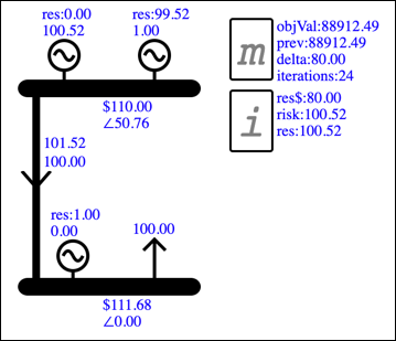
With reserves and losses enabled, solving the two bus model with the default Component properties gives the following result:
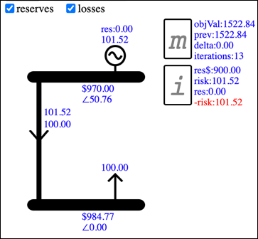
This shows a reserve deficit of 101.52MW associated with the Island Component. The Generator Bus price of $970 is due to the $900 cost of the reserve shortfall, combined with the $70 cost of the cleared energy offer.
Reserve Deficit
On the Data page for the Island Component i you can see the resCover Constraint, which requires that the islandRisk is covered by the islandRes and the islandResShortfall. There is also the islandResCalc constraint which calculates islandRes as the sum of cleared reserve on the Island's Generators:
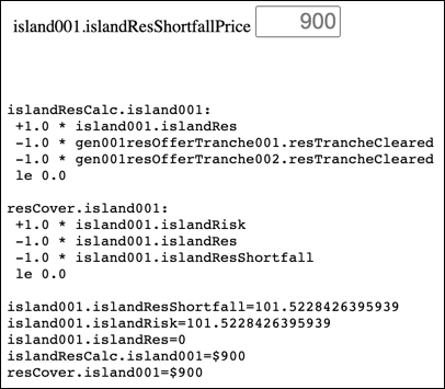
The islandRisk Variable is calculated by each Generator's islandFindRisk Constraint, as shown on the Generator Data page below. Hence the Island covers the largest risk.
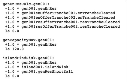
A Generator's risk is its cleared energy + cleared reserve. With no other Generator to provide reserve, the risk represented by the generation of the single Generator is covered by the Island's islandResShortfall Variable.
To produce a result that does not have a reserve Deficit we can either edit the Model Definition so that there is no requirement for reserve to cover risk, or we can add another Generator to provide reserve.
To add another Generator, click the Gen button. Then click Solve. In the new result shown below, each Generator provides some reserve to cover the risk presented by the other, and there is no reserve Deficit.
If you drag the new Generator down to the load Bus then all the generation will be scheduled there and all of the reserve scheduled at the other. This is because in this model the scheduling of reserve is not affected by losses.
Editing the Model Definition
The requirement for Island reserve to cover Generator risk is enforced by the Island resCover Constraint. Unticking the reserve option will remove this constraint from the model definition. You can see the model defition by going to the Main display and clicking the Model Def button. If you scroll down you can see the resCover Constraint definition, which will be unticked when reserves are disabled.
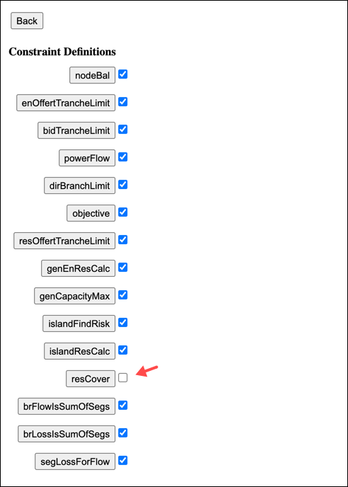
You can also see the islandFindRisk Constraint, which identifies the risk, and the islandResCalc Constraint which calculates the reserve cover. These do not need to be unticked because their only purpose is to calculate the Variables for use by the resCover Constraint.
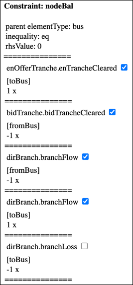
To see the details of a model definition, click on its button. For example the details of the node balance constraint defintion are as follows (when losses are disabled):
Reserve Price
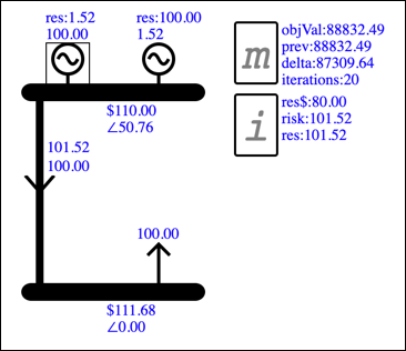
To explain the reserve price, build and solve the following model with reserves and losses enabled:
Note that the reserve price is $80, which is the value of reserve as represented by the shadow price of the resCover Constraint. To see this, add a Generator and edit its Data so that its energy offer limit is zero, its reserve offer limit is 1, and its reserve offer price is $0:
This will mimic relaxing the resCover Constraint, by allowing the constrained quantity to increase with no direct cost. Solve, and the result shows that the Objective Value has increased by $80:
Explaining the shadow price
Comparing the two results shows that relaxing the resCover Constraint by 1 unit has the following impact:
reduces by 0.48 units the reserve that gen002 was providing to cover the gen001 energy
reduces by 1 unit the reserve that gen001 was providing to cover the gen002 energy
provides direct cover for an extra 0.52 units of energy on gen001, which allows the energy on gen002 to be reduced by 0.52 units, allowing the reserve on gen001 to be reduced by another 0.52
Overall the value of 1 unit of reserve is that it supports the reduction of 0.48 + 1 + 0.52 = 2 units of $40 cleared reserve, benefiting the Objective Value by $80. Hence the shadow price of the resCover Constraint is $80, which sets the reserve price.
Any reserve that is offered will only clear if its offer price is <= the $80 benefit that would be obtained if it was free. You can demonstrate this by increasing the price of the 1 unit of reserve that has just been added... at $81 it will stop clearing.
Disabling Losses
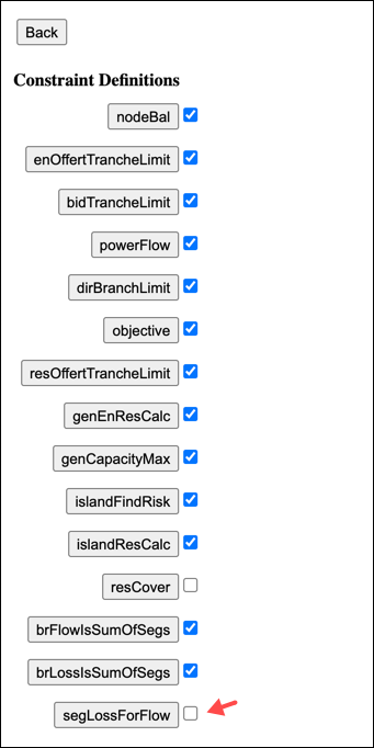
To see the constraints that are disabled when losses are disabled, go to the Model Def display. The segLossForFlow definition is un-ticked, thereby removing the link between branch losses and branch flow. This allows the branch flow Variable to increase without needing to also increase the branch loss Variable.
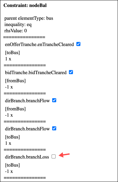
Clicking on the nodeBal Constraint you can see that the branchLoss Variable is removed from this Constraint. Branch losses are modelled as flow out of the Bus, and if the segLossForFlow Constraint is removed without removing this Variable then the solver can increase it to create extra load at the Bus when the Spring Washer Effect occurs:
Questions or Suggestions?
Send Email
Simplex Nodal
Director / Developer:
David Bullen

30 years in Electricity Industry (25 years in Electricity Markets)
BE Electrical
PGDip Operations Research
Cert Economics


Historical documents:
Operating Orders (Software I wrote when I was a Substation Operator)
Line Design (Software I wrote when I was a Graduate Engineer)